

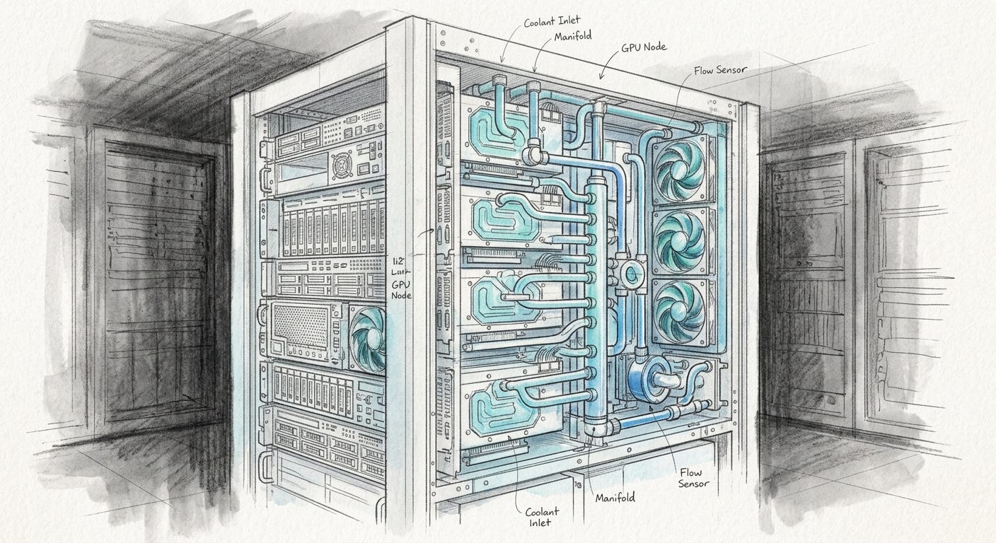
Image generation using Google Nano Banana.
I set out lately to try and find this out. For the uninitiated this meant sitting down to train my own Reinforcement Learning agent from scratch.
GPU consumption has been a pain point across the industry in the AI boom. GPU capacity is at a premium, and much of the cloud infrastructure we are used to is not fit for the new workload demands.
GPU cluster workloads for machine learning and deep learning are inefficient and fundamentally quite different from previous load balancing workloads at scale. Often suffering from bursty behaviour. The test was to support my own personal projects with a tool to assist with training models and also to help customers projects where appropriate. Since its such a hot topic across the sector with the AI boom right now it seemed an interesting problem to try and answer.
Algorithms compared against Maskable Proximal Policy Optimisation as part of the test. This may well not be the optimum RL approach to use. Nor do my experiments consider a lot of edge cases, failure scenarios etc. An experienced HPC infra engineer and data scientist would best guide this. Although I have had some initial review from people in my network.
Model training was executed in Google Collab notebooks and some scripting assistance from Claude Code/Cowork and Google Flash 2.5 I used synthetic data and a limited defined cluster configuration. I will post the script and details on Github for reference.
I started by considering what the agent can observe:
What would help a human make a good scheduling decision? Firstly the state of each GPU how much VRAM, utilisation and number of jobs running. So what we consider for server capacity more generally in cloud computing.
What can the agent do? So this is the state action space. Picking a GPU to send the next job to, or hold it in the queue if no suitable GPU is available.
Rewards - I decided just to focus initially on job completion, average utilisation and wait time. In server allocation you would want to optimise for roughly 60% to max 80% utilisation. Much more risks performance issues.
Comparing Reinforcement Learning with more standard algorithmic approaches.
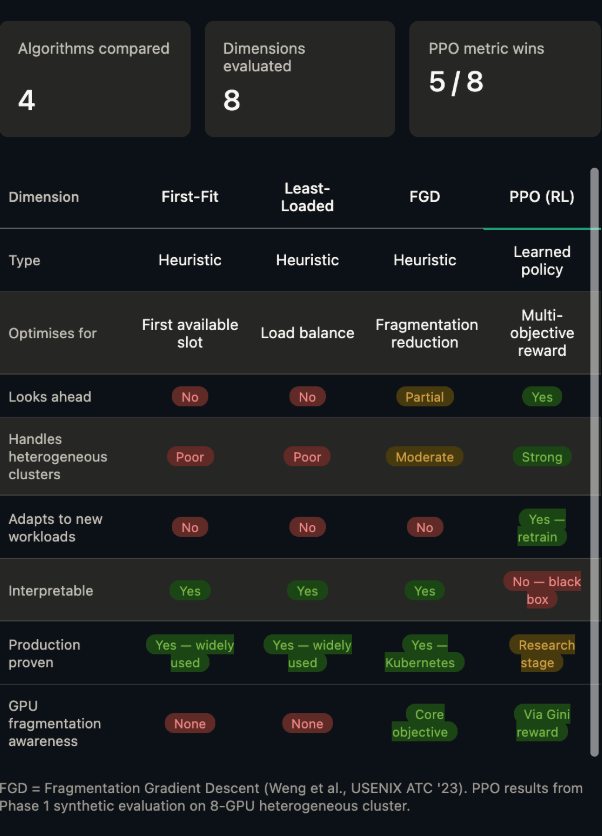
Structure of script to train the RL model.
Cell 1
Installs necessary Python libraries (gymnasium, stable-baselines3, sb3-contrib, tensorboard) using pip. - key ones are gymnasium, stable-baselines3 and pandas just for the final results table.
Cell 2
Keep Colab Alive - to prevent Colab timeouts - Contains a JavaScript snippet that sends periodic signals to the Colab backend to keep the notebook environment alive and prevent it from disconnecting due to inactivity.
Cell 3
Import all libraries and frameworks for the colab sheet - imports all the required Python modules and classes, including numpy for numerical operations, gymnasium for the reinforcement learning environment, stable-baselines3 and sb3-contrib for the PPO agent and action masking, pandas for data handling, and various callbacks for training.
Cell 4
Simulates the creation of a list of GPU jobs - Defines JOB_TYPES (configurations for different job categories like training, inference, batch) and the generate_workload function, which creates a synthetic list of GPU jobs with varied requirements (duration, VRAM, GPU count, priority) for the simulation.
Cell 5
Cluster configuration - number of servers/GPU’s and their size/type in the available cluster: Sets up the CLUSTER_CONFIG (describing the available GPUs and their VRAM capacities) and defines the GPU class (representing individual GPUs with methods for job assignment and state management) and the GPUCluster class (managing the collection of GPUs).
Cell 6
GPU Scheduler definition - Implements the GPUSchedulerEnv class, which is a custom Gymnasium environment. This class defines the observation space, action space, how the environment resets, how it progresses one step (step method), and includes helper functions like gini_coefficient for load imbalance and action_masks to restrict invalid actions.
Cell 7
GPU Scheduler environment - Performs a diagnostic check of the GPUSchedulerEnv to ensure it’s properly set up according to Gymnasium standards. It also measures the execution time of a single episode with random actions to gauge the simulation speed.
Cell 8
Defines baseline scheduling policies (first_fit_action for First-Fit and least_loaded_action for Least-Loaded), the evaluate_policy function to measure their performance, and then loads and evaluates the trained PPO (RL) model to compare its performance against these baselines.
Cell 9
Provides a more detailed diagnostic run of the First-Fit policy for a smaller number of jobs (20) and renders the environment state at intervals. This helps in visually understanding how the baseline scheduler performs.
Cell 10
Training the model - Configures and trains the MaskablePPO (Proximal Policy Optimization) agent. It defines mask_fn for action masking, make_env to create the training environment, and sets up callbacks (CheckpointCallback, EvalCallback) for saving models and evaluating performance during training. Finally, it initiates the model.learn() process.
Cell 11
Loads the TensorBoard extension and starts a TensorBoard instance, allowing visualization of the training progress (e.g., rewards, losses, episode lengths) that was logged to ./tb_logs/.
Cell 12
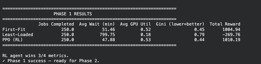
Model comparison and training results - Generates and prints a comparison table of the performance metrics (jobs completed, average wait time, GPU utilization, Gini coefficient, total reward) for the First-Fit, Least-Loaded, and PPO (RL) policies. It also includes a success check for Phase 1 based on how many metrics the RL agent ‘wins’.
Where Reinforcement Learning has an edge over standard algorithmic approaches for workload management.
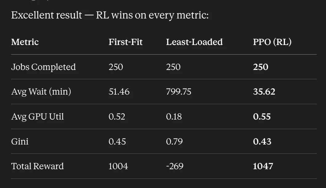
I started with just a small number of jobs 100 I then scaled this up to 250. Initial results looked promising, 35 min wait vs First-Fit’s 51 min is a 30% improvement. The agent has generalised well from 4 to 8 GPUs without any retraining on the new config.
Least-Loaded collapsed completely — 799 min wait and 0.18 utilisation could indicate a fundamental flaw. On a heterogeneous cluster, sorting by free VRAM causes it to repeatedly try routing large jobs to servers that can’t fit them, stalling the queue. This is exactly the kind of failure that heuristics are blind to and RL avoids.
Could RL be exposing a real weakness in a widely-used heuristic at scale? Well it is already understood that this is one of the limitations of the least loaded algorithmic approach, and engineers who manage infrastructure are skilled in where to apply it. However further validation is required to understand if this is really what is indicated here in terms of results or not.
I did not compare for Fragmented Gradient Descent a standard algorithmic approach in the initial tests. This will be considered in Phase 2.
Outputs and results from Phase 1 after several re-runs supported what was already established, however the issues with least loaded persist.
Right now cloud providers like AWS, GCP and Azure offer instance type selection at job submission time, you pick your tiers and pay accordingly. Workloads and appropriate algorithmic selection to manage them are also retrospective. You forward forecast infrastructure consumption based on what has already been demonstrated in your cloud environments. However what if the future is dynamic priority assignment where the scheduler itself infers urgency from job characteristics and cluster state in real time? Priority and consumption could be dynamically priced as well.
Having experimented enough to learn a bit about the approach I decided to make another experiment using sample cluster traces from the Cloud providers. Stay tuned for Phase 2.